
Create a dynamic table on Microsoft Excel It is not something too complex, the ideal is to start with the basics, this way it will be much easier. Thanks to pivot tables we find an interactive way to organize, group, calculate and analyze data. It is possible to manipulate this data in different ways to visualize exactly what we need.
Create recommended pivot table in Microsoft Excel
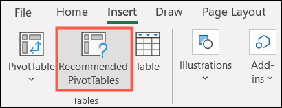
In the same way that we can insert a chart in Excel with the recommended chart options, we can also do this with a pivot table. For this we will have to go to the “Insert” tab and click on “Recommended pivot tables” on the left side of the ribbon.

Once the window opens, we will be able to see several pivot tables on the left. We’ll have to select one to see a preview on the right. If we see one that we want to use, we will have to select it and click “OK”.

This is when a new sheet opens with the pivot table we chose. We will also see in the right sidebar Fields of the pivot table which will allow us to edit the table.
Create our own table

If we want to create our own pivot table, we will have to go to the “Insert” tab and choose “Pivot Table” on the ribbon.
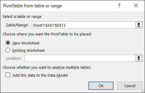
A new window opens, at the top, we will confirm the data set in the Table/Range box. Next, we will have to decide if we want the table in the new worksheet or in the existing one. To analyze multiple tables, we can check the box to add it to the data model. We will click on “OK”.

After this we’ll see the PivotTable and PivotTable Fields sidebar, ready for us to create the table or edit the recommended table we added.
Create or edit a pivot table
Using the PivotTable Fields sidebar, we’ll start by choosing the fields at the top that we want to include by checking the boxes. We can check and uncheck the boxes of the fields that we want to use at any time.
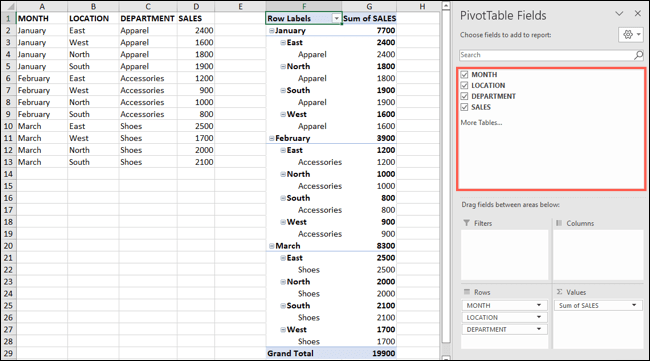
Excel then positions those fields in the boxes at the bottom of the sidebar, where it thinks they belong. This is where we can decide to position them where we want.

Depending on the type of data in the spreadsheet, we will see things like numbers in the Values box, dates and times, Columns and textual data, etc. These are the default values for these data types, but we can move them anywhere we want.

For example, if we want to see our months as columns instead of rows. All we have to do is drag that field from the Rows box to the Columns box and your table will update accordingly. Alternatively, we can use the dropdown arrows next to the fields to move them around.
If we have more than one field in a table, the order also determines the location in the pivot table. In this example, we have Department first and Location second in the Rows box, which is how they are grouped in the table.
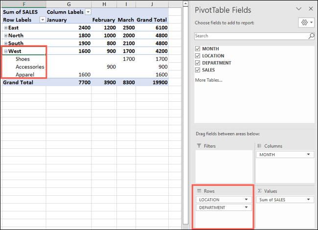
If we want to move Location over Department, we’ll need to see each of our locations as the parent fields, which is what we want. Then we simply use the minus and plus buttons next to each location so we can expand the group and see the departments.
Since it is possible to move fields between tables with drag and drop actions, we can find the best option for your data analysis.


