One small issue Google Sheets has is that it doesn’t automatically track character recall. So if we need count characters in a cell in Sheetswe will have to use the functions and formulas that we will explain how to use below, depending on the situation.
Count characters in a cell in Google Sheets
For this we are going to use the LEN function that works the same as in Microsoft Excel. It gives us the number of characters in a cell using a simple formula. The syntax of the function is LEN(text) where we can use an actual text or cell reference for the argument.
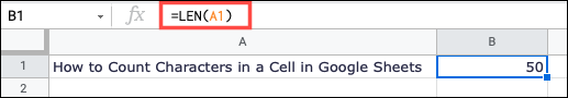
For example, in order to find the number of characters in Cell A1, we would have to use the following formula: =LEN(A1)
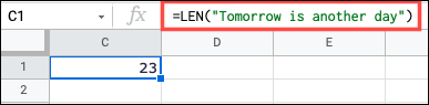
If we want to find the number of characters of a specific text, we will use the following formula, we will have to put the text in quotes: =LEN(«Tomorrow will be another day»)
Something very important that we must consider about the LEN function is that it is in charge of counting each character, among which are included: numbers, letters, simple spaces, non-printable characters and punctuation.
Count characters in a range of cells
There are many functions that allow us to use a cell range as an argument. The problem is that LEN is not one of these. Although we should not worry, we can make use of the SUMPRODUCT function to the LEN formula, to be able to count characters in a range of cells.

This function is responsible for calculating the sum of arrays or cell ranges. The syntax is SUMPRODUCT(array1, array2, …) where we only need the first argument.
For example, if we want to count in cells from A1 to A5, we will use this formula: =SUMPRODUCT(LEN(A1:A5))
Count instances of specific characters in a cell
One more adjustment we can make when counting characters is to count certain characters. Perhaps we want to know how many times the letter A appears in the text string of a cell. To achieve this we are going to use the SUBSTITUTE function.

We are going to see a practical example, then we are going to divide the parts of the formula. Here we will see the number of times the A will appear in cell A1: =LEN(A1)-LEN(SUBSTITUTE(A1,»A»,»»))
- SUBSTITUTE(A1,»A»,»») takes care of finding and replacing each letter A with whatever is between the quotes, in this case nothing.
- LEN(SUBSTITUTE(A1,»a»,»») counts the number of characters that are not the letter A (substituted).
- LEN(A1) as before, counts the characters in cell A1.
Finally, we have a minus sign that divides the formulas to subtract the second LEN formula from the first, giving us a result that is 3.
The main disadvantage of counting specific characters with this function is that it is case sensitive. Therefore, if we examine our text and ask ourselves why the result is 3 instead of 4, the reason is just that.
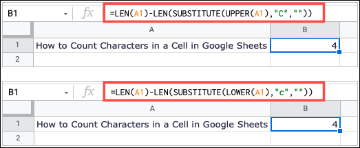
To get around that, we can add a new function to the formula. We can use UPPER or LOWER. So, in order to count all the times the letter A appears in the cell, we are going to use one of the following formulas.=LEN(A1)-LEN(SUBSTITUTE(UPPER(A1),»A»,»»))
=LEN(A1)-LEN(SUBSTITUTE(LOWER(A1),»a»,»»))
In case the text has too many capital letters, it is possible to use the first formula; if it’s mostly lowercase, we’ll use the latter. The idea is to use UPPER with the capital letter in quotes and LOWER with the lower case.

