
Microsoft Excel offers a built-in tool to classify our data. However, it is possible that, in many occasions, we need the flexibility that a function and a formula offer. In this case, we will see how use Excel’s SORT function with examples for better understanding.
One of the great benefits of the SORT function is the possibility of ordering the data in different places. If we need to manipulate certain elements without changing the original data set, then this sort function will be ideal.
On previous occasions we have taught you how to use different Microsoft Excel functions that are extremely useful on different occasions, such as: INDIRECT, CHAR, EXP, among others. We find it such a useful application that we even recommend knowing all the text functions to facilitate daily tasks.
About the Excel SORT formula
The sort formula syntax would be SORT(range, index, order, by_column) where the first argument is required. If we want to understand about the optional arguments, we explain it below:
- Index: we will enter a number to represent the row or column which we want to order. Excel sorts by row 1 and column 1 by default.
- Order: we will have to enter 1 for the ascending order, which would become the default if it is omitted, we can also add -1 for descending order.
- By_column – We’ll enter False to sort by row, which is the default if we omit it, True is to sort by column.
Using the SORT function in Microsoft Excel
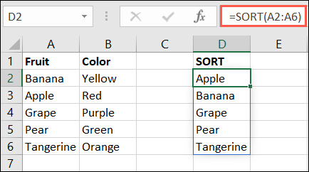
To see a basic example, we can sort the items in cells A2 to A6 using the default values for the optional arguments discussed above, here we’ll use =SORT(A2:A6)

If we want to sort on a larger range, we’ll include cells B2 through B6: =SORT(A2:B6). As we can see in the example, the elements will remain coupled with their attributes.

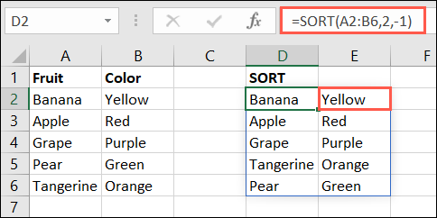
What we’ll do now is sort our range by the second column instead of the first. So we will have to enter 2 for the Index argument, which would be like this: =SORT(A2:B6,2)
What we will see now is that our articles are being arranged in ascending order by the second column, where green would come first, while yellow last.
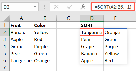
Now we will see how to use the Order argument to be able to sort our matrix in descending order where we will include -1: =SORT(A2:B6,,-1)
We must consider that we leave the argument Index empty. The reason is because Excel uses the first row and column by default.
In case we wanted to sort descending by the second column, we would have to use this formula: =SORT(A2:B6,2, -1)
Here we include a 2 for the Index argument and a -1 for the Order argument. So, we’re going to look at the yellow first and the green last.

To finish, we are going to give another example where we will include a value for each argument, in this way we can appreciate how they all work together. We’ll have to enter a larger array from A2 to C6, a 3 to sort by the third column, a 1 for it sorts ascending, and False to sort by row direction: =SORT(A2:C6,3,1,FALSE)
Thanks to the SORT formula, we can get a different view of our data depending on the order in which we want to see it. This makes it an interesting and useful data analysis tool.

