
It’s not complicated use the IMSUB function in Microsoft Excel, its purpose is to return the difference between two complex numbers. In this simple guide we are going to see how we can use this function.
How to use the IMSUB function in Microsoft Excel
The first thing we will have to do is start Microsoft Excel as usual, we will have to create a table or use a file that already contains the data that we want to use with the IMSUB function.
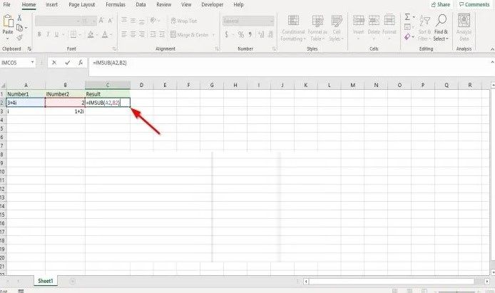
We are going to have to write the formula in the cell where we want to place the results “= IMSUB (A2, B2)” without the quotes and then press “Enter” to see the results in question.
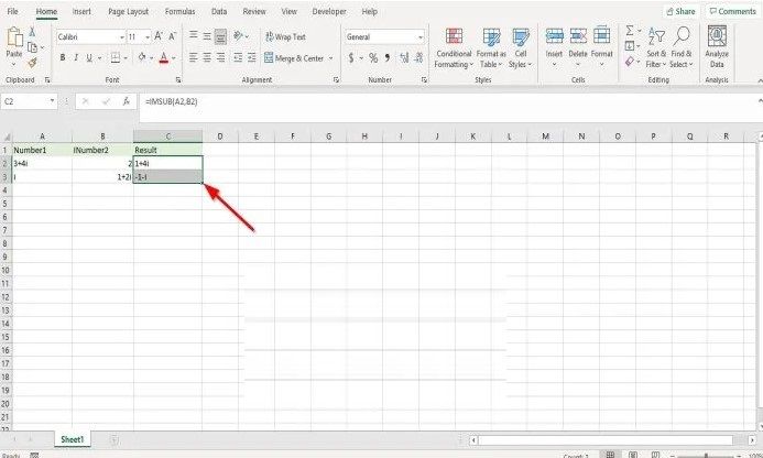
If we have more than one piece of data, what we can do is click on the result and keep it, then we drag it down to see the rest of the results.
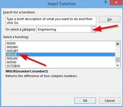
There are two more methods to be able to use this function. One of these methods is to click the “FX” button at the top left of the Excel spreadsheet.

“Insert function” will appear and we will have to search for “IMSUB” among all the functions. For this we will have to select one of the categories in the drop-down list, here we will have to choose “Engineering”. To continue, we will simply have to click on “Accept”.
Now a dialog box called “Function Arguments” opens.
- We will have to enter cell A2 of the input box in “Inumber1”.
- In the case of the entry “Inumber2” we are going to enter cell B2.
After this we are going to click on “Accept”.
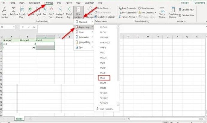
The other method is to click on the “Formulas” tab and then we will have to click on the “More functions” button in the function library group. After this we will click on “Engineering” and select IMSUB from the drop-down menu.
The “Arguments Function” will appear in the dialog box and we can use it without problems.


